A Simple Epigenetic Clock Using Python and SciKit-Learn
DNA methylation has emerged as a useful proxy for measuring the physiological state of an organism. DNA methylation is dynamic, changing over time in response to environmental stimuli, yet can also be stable for relatively long periods of time1. Thus, an individual who continuously lacked exercise and ate poorly for years would have an epigenetic profile that reflected this continued behavior. The dynamic yet stable nature of DNA methylation is extremely beneficial, maintaining information lost with more transitory signals, such as gene expression. This makes DNA methylation ideal for the development of biomarkers, which have already been developed to assess age 2,3 and BMI 4.
In this example we will use publicly available data from Aging effects on DNA methylation modules in human brain and blood tissue, 5 to fit an epigenetic clock using a penalized regression model. The data from this paper can be accessed at GSE41169. We will be working with the series_matrix_file deposited in GEO repository. The complete workflow will utilize several tools:
- SciKit-Learn; Several modules from SciKit will be utilized in this example
- Principal Component Analysis (PCA), used during quality control to identify and sample outliers
- Train Test Split, this provides a convenient way to split data into training and testing sets
- Lasso, Cross Validated, this is an implementation of a penalized regression model that we will us to generate an epigentic age model
- Pandas, this library will help us organize data for downstream analysis
- Numerical Operation Libraries
- Visualization libraries, to visualize quality control and the model output
Workflow
This workflow should be tailored to the data set and phenotype of interest, but the general process should be similar for many biomarkers. I start by setting up an analysis environment in Jupyter and pre-processing the data. After pre-processing the data we will perform quality control followed by fitting the epigentic age model.
Setting an Analysis Environment
After a jupyter instance has been created we will setup the analysis environment by import libraries and setting paths.
# set working directory where the series matrix data is stored
wd = 'path to working directory'

import pandas as pd
import numpy as np
import seaborn as sns
import matplotlib.pyplot as plt
from scipy import stats
from sklearn.decomposition import PCA
from sklearn.linear_model import LassoCV
from sklearn.model_selection import train_test_split
Pre-Processing Data
The raw data from GEO needs to be processed before a model can be fit. Pre-processing the data will change based on the input and phenotype of interest, however generalizable tools can be written to a handle diverse array of inputs. Once these tools are written, they are often imported into the jupyter environment and not written out in the notebook. However, for this example the tools are written out to highlight data pre-processing.
First we define an iterator that takes a text file line, processes that line and returns a list.
import gzip

class OpenSeriesMatrix:
    """Simple class to iterate over series_matrix_files
    Arguments:
        series (str): path to series file
    Attributes:
        self.f (object): read object
        self.process_line: decodes line if necessary and returns processed list
        self.__iter__: iteration method
        """

    def __init__(self, series=None):
        # if file ends with .gz open as a binary file, else open at txt file
        if series.endswith(".gz"):
            self.f = gzip.open(series, 'rb')
        else:
            self.f = open(series, 'r')

    def __iter__(self):
        with self.f as cg:
            while True:
                line = cg.readline()
                # if line is blank break loop
                if not line:
                    break
                yield self.process_line(line)

    def process_line(self, line):
        if isinstance(line, bytes):
            return line.decode('utf-8').replace('\n', '').split('\t')
        else:
            return line.replace('\n', '').split('\t')
Next we define how to store the data, identifiers present in the series matrix file are passed to the parser which then stores formatted data.
class SeriesMatrixParser:
    """Class to parse series matrix files into three components;
    file information, phenotype information, and methylation data.
    Arguments:
        series_matrix_path (str): path to series matrix file
        description_ids (list): list of identifiers for file descriptors
        sample_id (str): identifier for line listing sample names
        phenotype_ids(list): list of identifiers for phenotype information
        matrix_start (str): identifier list the start of the methylation matrix
    Attributes:
        self.series_matrix (OpenSeriesMatrix): iterator object
        self.series_description (dict): dict of file decriptors
        self.sample_ids (list): list of sample names
        self.phenotype_matrix {dict}: dict of phenotype information
        self.matrix_trigger (bool): bool to set beginning of
            methylation matrix in series matrix file
        self.matrix (list): list of methylation sites with values
        self.run (func): wrapper to get series matrix info
    """

    def __init__(self, series_matrix_path=None):
        assert(isinstance(series_matrix_path, str))
        self.series_matrix = OpenSeriesMatrix(series_matrix_path)
        self.series_description = {}
        self.sample_ids = []
        self.phenotype_matrix = {}
        self.matrix_trigger = False
        self.matrix = []

    def run(self, description_ids=None, sample_id=None, phenotype_ids=None, matrix_start=None):
        assert(isinstance(description_ids, list))
        assert(isinstance(sample_id, str))
        assert(isinstance(phenotype_ids, list))
        assert(isinstance(matrix_start, str))
        for line in self.series_matrix:
            if not self.matrix_trigger:
                self.get_descriptive_lines(line, description_ids)
                self.get_sample_ids(line, sample_id)
                self.get_phenotype_info(line, phenotype_ids)
                self.get_matrix(line, matrix_start=matrix_start)
            else:
                self.get_matrix(line)

    def get_descriptive_lines(self, line, description_ids):
        if line[0] in description_ids:
            try:
                info = self.series_description[line[0]]
            except KeyError:
                self.series_description[line[0]] = line[1:]
            else:
                self.series_description[line[0]] = info + line[1:]

    def get_sample_ids(self, line, sample_id):
        if line[0] == sample_id:
            self.sample_ids = line[1:]

    def get_phenotype_info(self, line, phenotype_ids):
        if line[0] in phenotype_ids:
            phenotype_label = line[1].split(':')[0].strip(' "')
            self.phenotype_matrix[phenotype_label] = []
            for phenotype in line[1:]:
                phenotype_split = phenotype.split(':')
                self.phenotype_matrix[phenotype_label].append(phenotype_split[1].strip(' "'))

    def get_matrix(self, line, matrix_start=None):
        if self.matrix_trigger:
            self.matrix.append(line)
        elif line[0] == matrix_start:
            self.matrix_trigger = True
We now want to initialize the classes above with our series matrix data, specifying the file lines we are interested in using line identifiers. The line identifiers are selected by manually inspecting the file. Additionally, we will transform the returned methylation values into a pandas dataframe and perform operations on the dataframe to simplify downstream analysis.
# name geo file
geo_file = 'GSE41169_series_matrix.txt'

# run parser class on the downloaded information, you will have to
# identify phenotype information and descriptors manually
example_matrix = SeriesMatrixParser(f'{wd}{geo_file}')
example_matrix.run(description_ids=['!Series_title', '!Series_geo_accession',
                                    '!Series_pubmed_id', '!Series_summary',
                                    '!Series_overall_design',
                                    '!Series_sample_id', '!Series_relation'],
               sample_id='!Sample_geo_accession',
               phenotype_ids=['!Sample_characteristics_ch1'],
               matrix_start='!series_matrix_table_begin')

# transform matrix list into a pandas dataframe
example_matrix_df = pd.DataFrame(data=example_matrix.matrix[1:-1],
                                columns=example_matrix.matrix[0])

# set index
example_matrix_df = example_matrix_df.set_index('"ID_REF"')

# transform strings to float values
example_matrix_df = example_matrix_df.apply(pd.to_numeric, errors='coerce')

# drop rows, methylation sites, with missing infromation
example_matrix_df = example_matrix_df.dropna(axis=0)
The final step of pre-processing is retrieving the phenotype of interest, in this case age.
# retrieve age phenotype
example_matrix_age = [int(x) for x in example_matrix.phenotype_matrix['age']]
Matrix Quality Control
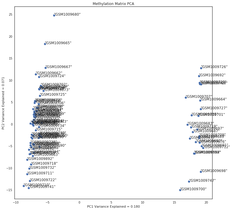
To ensure there aren’t large technical biases between samples, we will decompose the matrix using PCA then graph the output to check for outliers. If there are outliers we will remove them from downstream analysis.
# define a PCA object
qc_pca = PCA(n_components=4, whiten=False)

# fit the PCA object
qc_pca_values = qc_pca.fit_transform(example_matrix_df.values.T)

# get the variance explained for the first two principal components
variance_explained = qc_pca.explained_variance_ratio_

pc1 = qc_pca_values[:,0]
pc2 = qc_pca_values[:,1]
After decomposing the matrix we graph the matrix, and remove outliers based on a previous run.
# scatter plot of first two PCs, and retrieve and sample outliers
# list to store sample outliers
non_outlier_list = []
non_outlier_age = []
fig, ax = plt.subplots(figsize=(12,12))
ax.scatter(pc1, pc2,)
ax.set_title('Methylation Matrix PCA')
ax.set_xlabel(f'PC1 Variance Explained = {variance_explained[0]:0.3f}')
ax.set_ylabel(f'PC2 Variance Explained = {variance_explained[1]:0.3f}')
# iterate through pc1, pc2, and sample labels to add labels to plotted points
for x, y, label, age in zip(pc1, pc2, list(example_matrix_df), example_matrix_age):
    ax.text(x=x, y=y, s=label)
    # add outliers to list
    if x < 5:
        non_outlier_list.append(label)
        non_outlier_age.append(age)
plt.show()
Fit Penalized Regression Model
With the processed data in hand, a penalized linear regression model can be fit. First we want to dived our data into training and testing sets.
# want a list of sample names
sample_ids = list(example_matrix_df[non_outlier_list])

X_train, X_test, y_train, y_test = train_test_split(sample_ids, non_outlier_age, test_size=0.1)

# take dataframe values as a numpy array and transpose the array with .T
X_train = example_matrix_df[X_train].values.T
X_test = example_matrix_df[X_test].values.T
We then initialize and fit a penalized regression object, LassoCV, to the training data.
# initialize a penalized regression object
lasso_cv = LassoCV(cv=3, n_jobs=2)

# fit object
lasso_cv.fit(X_train, y_train)
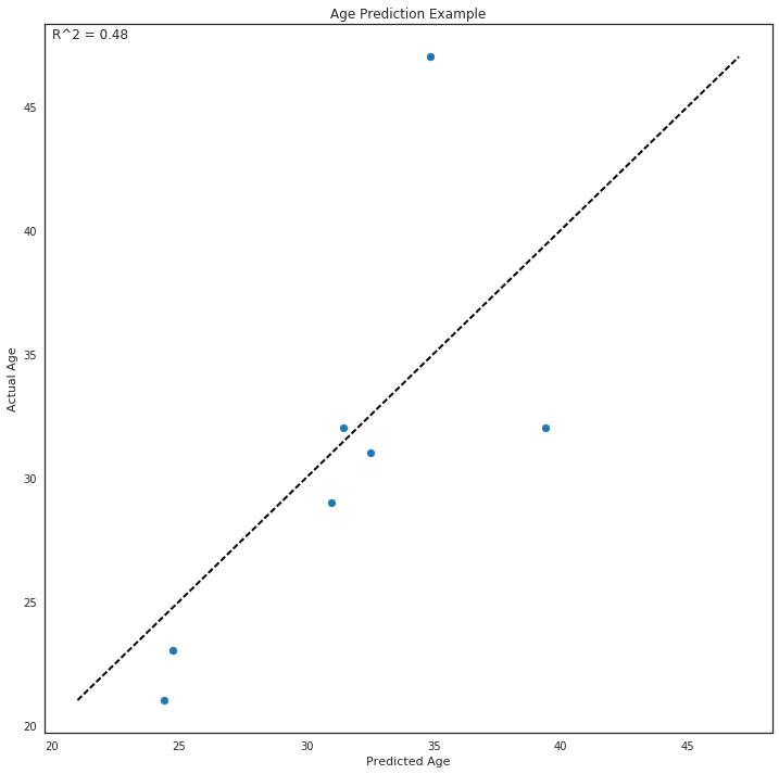
Score the Model
Using the testing data, we then predict the age using the methylation matrix and compare the predicted age to the actual age and score the model using Pearson’s R^2.
def r2(x, y):
    return stats.pearsonr(x, y)[0] ** 2

predicted_test_age = lasso_cv.predict(X_test)
test_score = r2(predicted_test_age, y_test)
Finally, we plot the model.
fig, ax = plt.subplots(figsize=(12,12))

ax.scatter(predicted_test_age, y_test, c=sns.color_palette("Paired")[1])
ax.plot([np.asarray(y_test).min(), np.asarray(y_test).max()],
[np.asarray(y_test).min(), np.asarray(y_test).max()], 'k--', lw=2)
ax.set_xlabel('Predicted Age')
ax.set_ylabel('Actual Age')
ax.set_title('Age Prediction Example')
ax.text(0.01, .98, f'R^2 = {test_score:0.2f}',  transform=ax.transAxes)

plt.show()
References
- Zemach, A., Mcdaniel, I., Silva, P. & Zilberman, D. Genome-Wide Evolutionary Analysis of Eukaryotic DNA Methylation. Science (New York, NY) 11928, science.1186366v1 (2010).
- Horvath, S. Erratum to: DNA methylation age of human tissues and cell types. Genome Biology 16, 96 (2015).
- Hannum, G. et al. Genome-wide Methylation Profiles Reveal Quantitative Views of Human Aging Rates. Molecular Cell 49, 359–367 (2013).
- Wahl, S. et al. Epigenome-wide association study of body mass index, and the adverse outcomes of adiposity. Nature 541, 81–86 (2017).
- Horvath, S. et al. Aging effects on DNA methylation modules in human brain and blood tissue. Genome Biol. 13, 1465–6914 (2012).